How To Add Values To A Vector In Matlab

MATLAB - Plotting

To plot the graph of a function, you need to take the following steps −

Define x, by specifying the range of values for the variable 10, for which the part is to be plotted
Define the role, y = f(x)
Call the plot control, as plot(x, y)

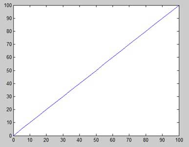
Following example would demonstrate the concept. Let us plot the elementary function y = x for the range of values for x from 0 to 100, with an increment of 5.

Create a script file and blazon the following code −

ten = [0:5:100]; y = x; plot(x, y)

When you lot run the file, MATLAB displays the following plot −

Plotting y = x

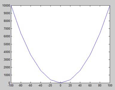
Let usa take 1 more example to plot the function y = x². In this instance, nosotros will describe ii graphs with the same function, but in 2nd time, we will reduce the value of increase. Please note that every bit we decrease the increase, the graph becomes smoother.

Create a script file and type the following lawmaking −

x = [1 2 3 four 5 vi vii 8 9 10]; 10 = [-100:twenty:100]; y = x.^2; plot(x, y)

When you run the file, MATLAB displays the following plot −

Plotting y = x^2

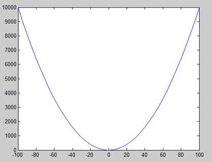
Change the code file a little, reduce the increase to five −

10 = [-100:v:100]; y = x.^two; plot(x, y)

MATLAB draws a smoother graph −

Plotting y = x^2 with less increment

Adding Championship, Labels, Grid Lines and Scaling on the Graph

MATLAB allows yous to add title, labels forth the x-axis and y-axis, filigree lines and besides to conform the axes to bandbox up the graph.

The xlabel and ylabel commands generate labels along 10-centrality and y-axis.
The title command allows you to put a title on the graph.
The grid on command allows you to put the filigree lines on the graph.
The axis equal command allows generating the plot with the same calibration factors and the spaces on both axes.
The axis square command generates a square plot.

Example

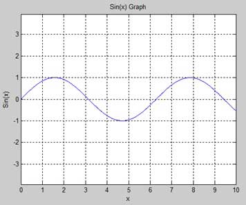
Create a script file and type the following code −

x = [0:0.01:ten]; y = sin(x); plot(x, y), xlabel('ten'), ylabel('Sin(ten)'), title('Sin(x) Graph'), grid on, axis equal

MATLAB generates the post-obit graph −

Sprucing up our graphs

Drawing Multiple Functions on the Same Graph

You lot tin can draw multiple graphs on the aforementioned plot. The following example demonstrates the concept −

Example

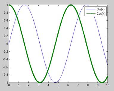
Create a script file and type the post-obit code −

x = [0 : 0.01: x]; y = sin(x); g = cos(x); plot(x, y, x, g, '.-'), legend('Sin(ten)', 'Cos(x)')

MATLAB generates the following graph −

Multiple Functions on the Same Graph

Setting Colors on Graph

MATLAB provides 8 bones colour options for drawing graphs. The post-obit table shows the colors and their codes −

Code	Color
w	White
one thousand	Blackness
b	Blue
r	Red
c	Cyan
g	Green
yard	Magenta
y	Xanthous

Example

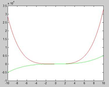
Allow united states draw the graph of two polynomials

f(10) = 3x^four + 2x^three+ 7x² + 2x + 9 and
g(x) = 5xⁱⁱⁱ + 9x + ii

Create a script file and type the following lawmaking −

x = [-ten : 0.01: 10]; y = 3*x.^iv + 2 * ten.^iii + 7 * x.^2 + two * ten + ix; g = 5 * ten.^three + 9 * x + two; plot(x, y, 'r', x, g, 'g')

When you run the file, MATLAB generates the post-obit graph −

Colors on Graph

Setting Axis Scales

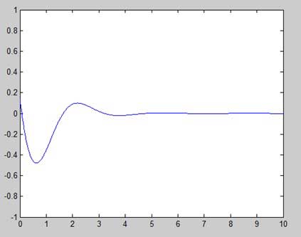
The centrality control allows you to set the axis scales. Y'all can provide minimum and maximum values for x and y axes using the centrality command in the following manner −

axis ( [xmin xmax ymin ymax] )

The following instance shows this −

Example

Create a script file and type the following code −

10 = [0 : 0.01: 10]; y = exp(-10).* sin(two*ten + 3); plot(x, y), axis([0 10 -1 1])

When you run the file, MATLAB generates the following graph −

Setting Axis Scales

Generating Sub-Plots

When you create an array of plots in the aforementioned figure, each of these plots is chosen a subplot. The subplot command is used for creating subplots.

Syntax for the command is −

subplot(g, n, p)

where, m and n are the number of rows and columns of the plot array and p specifies where to put a particular plot.

Each plot created with the subplot command tin have its ain characteristics. Following example demonstrates the concept −

Example

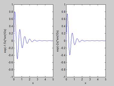
Let u.s.a. generate two plots −

y = e^−ane.5xsin(10x)

y = e^−2xsin(10x)

Create a script file and type the following code −

x = [0:0.01:v]; y = exp(-one.5*ten).*sin(ten*x); subplot(1,two,1) plot(10,y), xlabel('x'),ylabel('exp(–1.5x)*sin(10x)'),centrality([0 5 -one ane]) y = exp(-two*x).*sin(ten*ten); subplot(i,2,ii) plot(ten,y),xlabel('ten'),ylabel('exp(–2x)*sin(10x)'),axis([0 v -ane 1])

When you lot run the file, MATLAB generates the following graph −

Generating Sub-Plots